how to create a table array in excel

115 comments to "Excel array formulas, functions and constants - examples and guidelines"

Eda says:

Hello,

I have a column, in each cell consisting of many temperaments separated by commas. I need to find the mode based on the temperament. I don't want to convert text to columns.

Do you know any way to make this?

Thank you in advance!
- Hi!
  Unfortunately, without seeing your data it is difficult to give you any advice. Please provide me with an example of the source data and the expected result.
Paulus says:

Thank you for a very well written tutorial!
Dinesh says:

Many times whenever I could not find a solution of a problem, your web pages comes as saviour, Today also I learnt a good example from you index match array function. Thank you may god bless.
Darshna says:

Hi,
Can you please make format on Auto calculation regarding Sick Leave(SL),Casual Leave(CL) and Half day SL & CL,Automatically from Attendance on month wise?
Sari says:

Hi there, I have a complicated formula in place, I am using a defined array CustomerCode_=$D4$ as part of a wider SUMPRODUCT formula. However the cell $D4$ gives one option ie Customer A or Customer B or Customer C. I want to be able to have cell $D4$ reference Customer A AND Customer B as an aggregate. I defined a new array CustAGG_ for Customer A and Customer B CustAGG_ value is {Customer A; Customer B} and when I type CustomerCode_=$D4$ and $D$4=CustAGG_ it doesn't seem to work.

If I do it manually ie (CustomerCode_=Customer A)+(CustomerCode_=Customer B) I get the right series of 1 and 0 for the full array. However I have more than 2 customers and several aggregations to do so I am wondering if there's an easier way?
Amy Lackas says:

I don't know if Array is the way to go for this, but i have this data set the IDs are children of the Parent ID. Each row has a role type on it. What i need to do is determine for each Parent ID whether or not there was a TA or a Dev role. Any ideas on how to do this?

ID Role Type Parent ID
1001 BA 2001
1002 TA 2001
1003 Dev 2001
1004 QA 2001
1005 BA 2001
1006 BA 2002
1007 QA 2002
1008 BA 2002
1009 BA 2003
1010 TA 2003
1011 QA 2003
1012 BA 2003
1013 BA 2004
1014 QA 2004
1015 BA 2005
1016 TA 2005
1017 Dev 2005
1018 TA 2005
1019 QA 2005
1020 BA 2005
- Hello Amy,
  Supposing that your data are in columns A, B, and C, enter the following formula in cell D1 and then copy it down along the column:
  =IF(OR(B2 = "TA", B2 = "Dev"), "Yes", "No")
  
  Hope this is what you need.
Imran Masud says:

Svetlana!!
Actually you are a awesome lady. Many many thanks to you.
- - Imran Masud says:
    
    :) you are welcome
Barry Evans says:

Can I assign string variables in Selection.Formula array?

So, I am using an horizontal array, but have the values assigned to variables collected in VBA.

I need to change the code below so "A12" is str_ID and "04/11/2019" is dtm_date and "Sarah" is str_Name

Range("B3:D5").Select
Selection.FormulaArray = _
"={""A12"",""04/11/2019"",""Sarah""}"
Prasath says:

Hi Svetlana,
I have a challenging requirement. I need to compute ageing of Invoices paid. There are 3 dates involved. Payment date[1] (-) Resolution date[2] is age of the line. If Resolution date is blank, then the the formula should consider Invoice date[3]. I can do it easily in the sheet by using if(res date="blank",Inv date,Res date) and then put a count in cell on the numbers between 0-30, 30-60 etc. But I cannot add a new column in the file as it is a protected file. Can I build a formula for this. Can you please help.
Mohammed says:

hello,
I need help regarding matching two databases and returning a non-exact value based on a reference value. the first database (sheet 1) is:
Patient Number diagnosis
123321 Hypertension
112233 heart Failure
995566 Diabetes

the second database (sheet 2) is
Patient Number diagnosis
123321 Hypertension stage 1
112233 intrinsic heart Failure
995566 Diabetes mellitus

so as you see, the patient number is the common value of both sheets, but the diagnosis is not exactly the same, is there a way to make excel bring the approximate value (like if 5 or more letters matching) from sheet two and add it as an extra column to sheet 1, as a new cell in the same raw of the same patinet number...

Appreciating your help
Ankur says:

I have a paragraph in Cell A1 & A List of Text strings in Range E1:E100.
I want to put matching text string from E1:E100 to "1st to nth cell in cloumn C

Can you help.
Naman Nishant Rana says:

i have a range of values in the form of "from" and "to" and corresponding to that some quantities, call it array 1. I have another set of values in the same form of "from" and "to" but are the different from the first array, call it array 2. I need values corresponding to array 2 from array 1 by splitting the quantities corresponding to array 1 by dividing the quantities by difference of "from and "to" in array 1.
Tim says:

Nice article. Keep up.
Brett Pigon says:

I want to curve fit data with a quadratic polynomial, outside of trendline in plotting. Online sources suggest Linest(Y's,X's^{1,2},1,1) entered as an array formula while 3 cells are selected. I am using Office 2016. This results in the VALUE error all 3 cells. If the exponent instead points at an array variable, e.g. {1,2} entered as an array across two cells, Pointing at the first of the 2 array variable cells gives a valid slope and intercept in two cells, the N/A in the third. Pointing at the 2nd cell of the array formula, it looks like a quadratic fit but still 2 terms, the 3rd with the N/A. Ideas? Thank you.
Don says:

I need to copy down a constant column value (column 1) to an existing sum array?:

Selection.Subtotal GroupBy:=1, Function:=xlSum, TotalList:=Array(9, 10, 11 _, 12, 15, 16), Replace:=True, PageBreaks:=False, SummaryBelowData:=True
Orkhan says:

Hi All,
I have a question, not too advanced in excel, but to certain degree. I have a following table:
Column C - I have dates
Column I - I have number of students in training
I need to show in cell K1 the number of students who are in training this week. I came up with a long formula below which does the job, however is long and confusing for others. My question, is there a simpler way to show this by using TODAY and WEEKNUM via array formula or something more simpler than my current string below:

=SUMIFS($I$31:$I$78,$C$31:$C$78,">="&(TODAY()-(WEEKDAY(TODAY(),2))+1),$C$31:$C$78,"<="&(TODAY()+(7-(WEEKDAY(TODAY(),2)))))

Thanks!
Orkhan
Todd says:

I would like some help, can text from a drop down have a numeric value in a formula. Example 1-Year is the text and the value would be .85. So when I have a formula it would take the .85 x other values? Thank you
Laura says:

Thank you so much, you are a very good teacher =)
Kireiko says:

Timesheet Data Help
Hi there! Is there a way to pull data from an excel timesheet that would show who works what shift? My Timesheet is based off of approx 30+ people working various shifts (D or N) on a given day. I would like to be able to see who is working a Day shift on a particular day and conversely a N shift on that same day. I would like to see this data tallied somehow near the end of the timesheet as i already have it set up to count how many people are working a Day shift or N shift but I would like to see the names of the individuals pop up somewhere near the bottom of my timesheet (as a column list not in row format). Is this possible?

An example:

Employee Name:
a D D N N
b D D N N
c D D N
d D D
Day 1 2 2 2 1
Night 1 2 2
(i would like the name of 'a' to show up here - as a table or pop-up somehow?)
same but for both 'a' and 'b'
same but for 'b' and 'c'
I would like the names of 'a' to show up here for nights somehow
same but for 'a' and 'b'
(the start of the above comments indicate the cell location it would have shown up on my excel worksheet but pretend the first three comments are on the same row and the last two are on the row below)
I mean, i *could* do it manually, but that seems really tedious and I'm sure excel has some function to do this for me. I'm just not smart enough to put it together, Lol. I'm thinking vlookup is involved but i'm not sure how to set up my formula right.

Any help is greatly appreciated!

Thank you!

(Ive already posted this to the microsoft help comm forum and theyve already helped me with a VBA script. I am just wondering if there is a formula that can do this same thingÉ)
sarita says:

Example 1. A single-cell array formula
how it is "20" ? , i got the answer 45
- Hi Sarita,
  
  Maybe you have different source data? You can try subtracting the numbers in column B from column C with a simple formula like =C2-B2, and see if any difference equals 45.
Shubham singla says:

If i use or function in front istead of using + sybomls between them can they again give same result
Kathe says:

My Spreadsheet looks like this:

Column Column Column Column Column Column
A B C D E F
2018 2017 2016 2015 2014 2013
1.Link * * * * *
2.JetPro W * * W
3.G&G W W W W W
4.MDBA
5.Bill G. W W W W

Column A; contains the names of the current year winners
Columns B-F; shows there status from Previous years
'*' denotes Honor roll status for that year
'W' denotes they were on the winner list for that year
'a blank cell' they did not make the list that year

In order to receive 'honor roll(*)' it must be their sixth consecutive year on the winners list.

I am trying to write a formula that will highlight 'Column A' to show their status for the current year.
RED highlight for 'new honor roll'
Blue highlight for 'repeat honor roll'
Yellow Highlight for 'new winner'

For Example, referring to the chart above:

#1: Blue Highlight - b/c they have been on honor roll for >6 yrs. consecutively
#2: No Highlight - b/c they lost there status in 2016, so only have 2 consecutive wins (2017&2018)
#3: RED Highlight - b/c 2018 makes their 6th consecutive win; they move to Honor roll status 'new honor roll'
#4: Yellow Highlight - b/c they were not on the previous years winners list
#5:Yellow Highlight - b/c they were not on they previous years winners list
Manish Pandey says:

Hi,

Thank you for this information. I was finally able to solve my problem after going through your tutorial. I did not find here solution to exact problem i was having, but still, applying things taught here, I was able to do it.

Problem: To count number of rows where values in one column (Say A1:A100) is greater than the corresponding values in other column (Say B1:B100).

My Solution is as follows:

{=SUM(IF((A1:A100)>(B1:B100), 1, 0))}

Thanks a lot. Regards.
Kevin says:

I have an array formula in a VBA routine covering several rows.
I need to copy the VALUE resulting from executing the array formula into another column on the same sheet. However, copy and paste or even paste special values does nothing.

What's so special about getting the values only from an array formula under VBA?
Jugh says:

Hi, i just tried to edit the =SUM(LARGE(range, {1,2,3})) array formula to
=LARGE(range,{1;2;3}). The idea was to get it to list the 3 largest numbers when i dragged the original cell down 2 cells.

Unfortunately it only displays the biggest number meaning it was only reading the 1 and not the 2 or 3. So it didn't matter how many times i dragged the cell down it would only show me the biggest number.

Can someone explain to me why? , from my understanding i assumed it would naturally follow the constants from 1 to 3 when dragged down, thus giving me the first largest to 3rd largest numbers.
SD says:

Hey Doug - Its actually the second screenshot in this post.
Please check this section "Simple example of Excel array formula".

But anyways, found a way using :

=IF(IFERROR(FIND("30",INDIRECT(CONCAT(CHAR(64+MATCH("Sold",1:1)),ROW(E2))))>0,FALSE),INDEX(A:A,ROW(E2)),"")

So basically , E2 will now have the value at A2,if column SOLD as value 30 in it, dragging the formula down and will repeat it. (need adjustment to 1:1 or use formulas -> name manager to create a named value).

Thanks for your help !
SD says:

How I can find all products where sold=30 ?
- Doug says:
  
  SD:
  The function to use is the SUMIF function. Where the values to sum are in the range B27:B32 and the values to sum are equal to or greater than 30 the formula is:
  =SUMIF(B27:B32,">=30")
  If the values to sum are only the ones equal to 30 then you just have 30 and no double quotes. =SUMIF(B27:B32,30)
  Use the COUNTIF function in the same way to get the number of products sold. So the formula would look like: =COUNTIF(B27:B32,30)or =COUNTIF(B27:B32,">=30")
  - SD says:
    
    Thanks Doug, But that gives me 60, I want to see "Kiwi , Mango"
    - Doug says:
      
      SD:
      Can you post a copy of the columns your data is in?
      It'll help if I can see what you're working with.
Neeraj Sharma says:

Hi ,

I have the data in below format:

A -100
B -234
C -32

A -123
B -221
D -456

A -145
B -245
C -312
D -478

I want to format this data as:
A B C D
100 234 32
123 221 456
145 245 312 478

Could you please help me how it can be done in excel?
- Doug says:
  
  Neeraj:
  In working briefly with your example data the only thing I can come up with is a procedure that involves Text-to Column then copy and transpose. If you have a lot of data like this, it will be a time consuming major pain to get the job done, but it can be done. Because your data is not in a consistent structure I can't figure out another way to do it without resorting to some code. Even then it would not be easy. Anyway, here's the way it can be done:
  Select each group of the data for example the first three numbers.
  Then under Data choose Text-to-Columns.
  Then, choose the Delimited button then next.
  Then, check the Other box and enter a hyphen in that field, then highlight the first column that contains the letters and choose the Do Not Import button, then Next.
  Now the numbers will be in separate columns. Select these three cells, copy them and then choose Paste Special and select the Transpose button.
  Click Paste and the numbers will be in three separate columns which you can put headers on A,B and C. Go Ahead and put a header on a fourth column as D.
  You'll have to go through this same procedure for each of these with the exception of the second group of data.
  With this group after you've got it in the separate cells, you'll need to just copy the top two numbers and transpose them into the proper cell and then copy the last number into the D column by itself.
David says:

This is very helpful, but I'm struggling with extending it to my application.

I need to see how many hours exist for each person in a month, and then use that person's employee number, look up his (or her) rate, and then multiple total hours by that person's rate -- and then I need to do this for each person who charged that month...to figure out the total cost for that month.

Here is example data:

Emp # Name Rate
11111 John 175
22222 Paul 150
33333 George 125
44444 Ringo 130

May June July
Proj 1
John 10 10 10
Paul 15 20 30
Proj 2
John 11 22 33
George 33 40 40

Proj 3
Ringo 16 22 44
George 44 44 44

xxxx

So, I'd look up John's rate and then multiple it by 22 hours and then George's rate and multiple it by 77, and do this for each row...and then sum up those products.
Frank says:

Very nicely done tutorial. Easy to follow with good progression of complexity from example to example.

Thank you.
Mark says:

Hi, I have a spreadsheet for monitoring athletes training. In this I collect the type of training (running, cross-training, gym), how long they trained for (in minutes), and the intensity of exercise (training zones from 1-10). I want to calculate the total "training stress". Normally, this would simply be time multiplied by intensity. However, the training zones are non-liner; zone 4 is not twice as hard as zone 2, zone 10 is not 2.5 times as hard as zone 4. Also, each type of exercise has a different effect. Zone 10 running is harder on the body than zone 10 cycling. I know the exact multiplier for each zone of each sport, I just don't know how to create a formula that will check the exercise type, intensity type, and then multiply by the training stress factor.

The training stress factors are as follows:
Running: 0.17, 0.25, 0.33, 0.50, 0.67, 1.00, 1.33, 1.67, 2.08, 2.50
Cross training: 0.08, 0.13, 0.17, 0.25, 0.33, 0.50, 0.67, 1.00, 1.33, 1.67
Gym: 0.02, 0.04, 0.08, 0.13, 0.17, 0.25, 0.33, 0.50, 0.67, 1.00

So, if I did 60 minutes of zone 4 running (stress factor 0.50), the training stress is 60mins * 0.50 = 30

If I did 60 minutes of zone 4 cross-training [e.g. cycling] (stress factor 0.25) the training stress would be 60mins * 0.25 = 15.

I hope that makes sense.

In my spreadsheet I am inputting the following data: date, training type (run, cross-training, gym), training zone (1-10). I then want to have a final column that calculates the training stress by identifying the training type and training zone, and then multiplying the training time by the training stress factor to give the total training stress.

Does this even make sense, and is it possible?

Thanks
- Hi Mark,
  
  Your task is quite interesting. I'd recommend you first to create a small table that will contain the stress factors for different types of training like the one below:
  
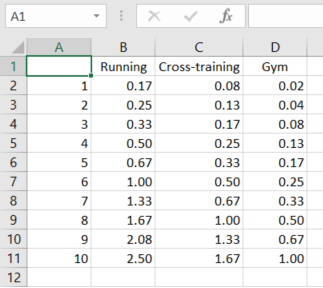
  Suppose this table is placed on Sheet 1, and your table where you are inputting the data is on Sheet 2:
  
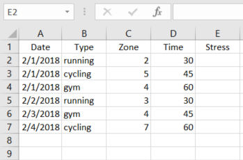
  Then please enter the following formula into cell E2 in the table on Sheet 2:
  
  =INDEX(Sheet1!$A$1:$D$11, MATCH(C2,Sheet1!$A$1:$A$11,0), MATCH(B2,Sheet1!$A$1:$D$1,0))*D2
  
  You'll get the total training stress for a particular activity type:
  
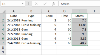
  If you want to get the stress summary by date, then please use the standard Excel Subtotal feature (Data -> Subtotal).
  You can find more information about INDEX and MATCH in this article on our blog. To see how to use the Excel Subtotal feature, please go here.
  
  I hope this information will be helpful for you.
Thabang says:

Good day. Can some assist. which function is used to auto fill these sheet on the dates side. I need short cut on my excel to auto fill the dates like that I only know control D which is time consuming.
25-Oct-17 Stopped 1203
25-Oct-17 Stopped 1203
25-Oct-17 Stopped 1203
25-Oct-17 Stopped 1203
26-Oct-17 Stopped 1203
26-Oct-17 Stopped 1203
26-Oct-17 Stopped 1203
26-Oct-17 Stopped 1203
27-Oct-17 Stopped 1203
Stopped 1203
Stopped 1203
Stopped 1203
28-Oct-17 Stopped 1203
Stopped 1203
Stopped 1203
Stopped 1203
Stopped 1203
29-Oct-17 Stopped 1203
Stopped 18
Stopped 3001
Stopped 3010
30-Oct-17 Stopped 18
Stopped 3001
Stopped 3010
Stopped 3011
Stopped 3012
- Hello,
  
  We have another article that describes how to fill empty cells in your table. Please have a look at it.
  
  Hope you'll find it helpful.
udaya says:

Hi Sir,
I have a data base, It includes columns A to J. From A- Name, Item Ref: Product, Location, Qty, Delivered Qty, Request date, Promised Date, etc.

Under Name there are more customer names and one customer name has more than one records.
Then how can I get displayed all the records related to a customer in a different sheet.
Ex. If I type the customer name Ann in a different sheet, then I need to see all the records available under Ann.
So what is the formula that helps me.

Thanks,
Udaya.
Kuze says:

There is a mistake made in the post. The * is not the logical AND operator when used in array functions. It is simply that the Boolean values when used in arithmetic operators are automatically converted to numeric equivalents. So the section on AND and OR functions is wrong. Take for example the following formula presented in that section:
=SUM((A2:A9="Mike") * ( B2:B9="Apples") * ( C2:C9))

The "A2:A9="Mike"" returns a Boolean which is then converted to a numeric when it is multiplied with "B2:B9="Apples"" which in return is multiplied to "C2:C9". When both "A2:A9="Mike"" and "B2:B9="Apples"" are true, the corresponding value from "C2:C9" is taken into the sum calculation. The expression looks as follows 1*1*C.
- Hello Kuze,
  
  It is true that when the logical values of TRUE and FALSE are used in arithmetic operations, they are converted to 1 and 0, respectively. But it is also true that in array formulas, multiplication acts as the logical AND function because it follows the same rules as the AND operator. That is, multiplication returns TRUE (1) only when all of the elements are TRUE. If any of the elements is FALSE (0), the result is FALSE (because multiplying by 0 always gives zero).
  
  On the other hand, addition acts as the OR operator because it returns TRUE (>0) if any of the elements is TRUE. And the result is FALSE (0) only when all elements are FALSE.
Larry says:

I am just not grasping how to get the formula I want, though I know the answer is in there. I want to have a formula look up a specific item (say 'sam's apples) and then fill in the corresponding rows with the last year's sales by month. In other words (currently):
a b c d e
Company Jan Feb March April
1 Sam's apples

2

3

What I want once it pulls the data from a separate spreadsheet:

a b c d e
Company Jan Feb March April
1 Sam's apples $532 $225 $632 $1032

2

3

I have over 2000 rows to sort and the company and the sales $ do not match up. Thanks ahead-
manoj hayaran says:

i want to create this type of table to sort the data
col A B c
type weight colD E F G H
Gr-1 Gr2 1000 Gr1 Gr2 Gr3 Gr4 up to Gr17
Gr2 Gr3 2000 Gr1 1000 4000
Gr3 Gr4 3000 Gr2 2000
Gr1 Gr3 4000 Gr3 3000
up to Gr17 please help
Daniel says:

Светлана, спасибо за такую развернутую статью, наконец-то исчерпывающее объяснение про формулы массивов!
SST says:

I need to display name of students separated with Comma in one cell holding same grade.
ljubo says:

Hello everyone!
Dear Svetlana, how to Sum numbers from array of text cells? textNUMBERtext A1:D100

This working with single cell: =LOOKUP(99^99;--("0"&MID(A1;MIN(SEARCH({0\1\2\3\4\5\6\7\8\9};A1&"0123456789"));ROW($1:$1))))
Help please :)
Hank says:

Does anyone know how to solve this problem?

I want to be able to provide a validation list for a lot of the fields in my workbook. I want to only use 1 formula for all the validation lists.

My workbook has at least 8 sheets in it. One of those sheets is a definition sheet and it lists the names of each worksheet, the column header name, and a description of what I use the column for and has indicators as to whether or not the column should be validated with a list. If so, the list I want to be comprised to validate the cell would come from the contents of the definition sheet.

Here is sample data from the definition sheet.
| A | B | C | D | E
--|-----------|----------|-----------|-------|-----------
01| SheetName | ColTitle | ValueType | Value | Definition
--|-----------|----------|-----------|-------|-----------
02| DataEntry | Fruit | Selection | Apple | An apple that can be eaten
--|-----------|----------|-----------|-------|-----------
03| DataEntry | Fruit | Selection | Orange| An orange that can be eaten
--|-----------|----------|-----------|-------|-----------
04| DataEntry | Fruit | Selection | Pear | A pear that can be eaten
--|-----------|----------|-----------|-------|-----------
05| DataEntry | HasSugar | Boolean | Yes | Answer positively
--|-----------|----------|-----------|-------|-----------
06| DataEntry | HasSugar | Boolean | No | Answer negatively
--|-----------|----------|-----------|-------|-----------
07| DataEntry | Calories | Numeric | | Indicates number of calories

On the DataEntry Sheet I have the following
| A | B | C |
--|-----------|----------|-----------
01| Fruit | Calories | HasSugar |
--|-----------|----------|-----------
02| | | |
--|-----------|----------|-----------|

I want to click on the Validation option in the Data Tools area of the Data ribbon and enter the same formula for cells A2 and C2. I will select Data Validation and in the Data Validation dialog box I would select List. What I need is a formula to insert in the Source field that will be the exact same formula every time on every sheet.

I think I can do this using VBA by calling a function that I would create but I was wondering if an array function or set of array functions already exist to accomplish this.

Basically, if I used a VBA function to do this, the function would:

1. Accept 2 parameters: SheetName and ColTitle.
2. It would create a range for the entire Definitions Sheet
3. A blank return string would be initiated.
4. A For Each row loop would be used to span all the rows in the sheet range
5. IF would compare the SheetName and ColTitle fields for a match
6. If would compare if the ValueType was Selection or Boolean
7. If the length of the return string > 0 a comma would be added
8. The matching value field would be added to the return string
9. Loop
10.Return the return string.

The Return String would contain a commas separated list of values.

Example: If I named the Function GetValidationList() and called it like so:
GetValidationList( MID(CELL("filename",A1),FIND("]",CELL("filename",A1))+1,255),
INDIRECT("R1C" & COLUMN(),FALSE) ) from cell A2, it would send "DataEntry", "Fruit" to the function and get back "Apple,Orange,Pear". If I called it using the exact same information from cell C2 it would send "DataEntry", "HasSugar" to the function and get back "Yes,No". These return strings would cause me to have pull down menu so that I can select the answer for Fruit or HaSugar.

I am wondering if there is any formula I can use other than having to write the VBA function that would allow me to do this as well.

My thoughts are if there was an array function that I could tell it the range of the Definitions spreadsheet to look at, filter the range by 2 fields "SheetName" and "ColTitle", and return an array of the matches, that it might perform the validation task much quicker than it takes for VBA.

Let me know your thoughts.

Thanks.
Jiri says:

Hello, can someone please help me figure out why the following arrayformula works

={OFFSET(INDIRECT("'GEN rates'!E"&MATCH(RIGHT(tool!K23,2)&A2&tool!F21,'GEN rates'!A68:A79&'GEN rates'!B68:B79&'GEN rates'!C68:C79,0)),ROW($A$68)-1,0)*(tool!M23-tool!H23)+OFFSET(INDIRECT("'GEN rates'!E"&MATCH(RIGHT(tool!K23,2)&A2&tool!H21,'GEN rates'!A68:A79&'GEN rates'!B68:B79&'GEN rates'!C68:C79,0)),ROW($A$68)-1,0)*(tool!M23-tool!F23)+IF(RIGHT(tool!K23,2)="EU",(tool!G23+tool!I23)*'GEN rates'!E80,0)}

while the following one with nested IF returns Value# error?

={IF('GT support'!B11<3,OFFSET(INDIRECT("'GEN rates'!E"&MATCH(RIGHT(tool!K23,2)&A2&tool!F21,'GEN rates'!A68:A79&'GEN rates'!B68:B79&'GEN rates'!C68:C79,0)),ROW($A$68)-1,0)*(tool!M23-tool!H23)+OFFSET(INDIRECT("'GEN rates'!E"&MATCH(RIGHT(tool!K23,2)&A2&tool!H21,'GEN rates'!A68:A79&'GEN rates'!B68:B79&'GEN rates'!C68:C79,0)),ROW($A$68)-1,0)*(tool!M23-tool!F23)+IF(RIGHT(tool!K23,2)="EU",(tool!G23+tool!I23)*'GEN rates'!E80,0),"incl.in FOB")}

I have been racking my brains to no avail so far, and seek any kind of advice to make the array formula work under the additional IF condition in the second case (otherwise the formulas are the same)

Many thanks in advance,
supritha says:

how to give an array as input?
- Giovanni Ciriani says:
  
  just name a range, and use the range name as input.
eon says:
Dutch says:

In the first example you say the grand total can be calculated with "=SUM(B2:B6*C2:C6)" but this should actually be "=SUMPRODUCT(B2:B6*C2:C6)"
- Hi Dutch,
  
  This can actually be either, array SUM or SUMPRODUCT, which is an array formula by its nature.
Jeff Lucas says:

Hello,

I need some help with calculating percentiles while using an array formula. Current formula is:

=IF(B7:B15>6,PERCENTILE(IF(Data!$G:$G=ReportPages!A1,IF(Data!$E:$E=ReportPages!A7:A15,IF(Data!$I:$I>0,Data!$I:$I))),0.1),"*")
ENTER +CTRL + SHIFT

The return value is #N/A

I isolated the issue to the "ReportPages!A7:A15" portion of the formula. It works fine with I change this to reference a single cell. Any help would be great.
Rachid says:

Hi Svetlana;

Think you for your efforts to make learn Excel tools.I would like to Know if i can put for example {1; 2; 3} in the rows of the Offset function,and what it happened if i had put it and used all formula in sum function.

Best Regart
Mike says:

Wow!

Am in love with your articles. Very easy to understand.

I dreaded working with arrays initially.

Thanks for putting a smile on my face:-)
Pavan says:

i have data in that i need to lookup 2 values matching data should on third cell and its duplicate data, suppose the data like

DATA
Product mm/dd/yyyy mm/dd/yyyy Sales
apples 11/10/2015 11/11/2016 20
oranges 11/10/2015 11/11/2016 52
banana 11/10/2015 11/11/2016 35
apples 11/10/2013 11/9/2015 66
oranges 11/10/2013 11/9/2015 69
oranges 9/8/2012 10/10/2013 55

Result data would be below

Product Date Required result
Apples 11/11/2014 66
Orange 9/9/2013 55
Danica Rose Oc says:

I am currently doing a project in excel, it is a database for medicine with a running lot no. which means a lagundi table can have many lot no. w/c is based on the date it is produced, now i want to display in the sheet what are the list lagundi with a specific lot no. which first entered the warehouse that has a quantity availble so it is easy to locate? WHAT WILL I DO WHAT FORMULA, HELP ME PLEASE IF I CANT SUBMIT THIS IT IS A FAILING GRADE THAT AWAITS ME. THANK YOU
Uche Uche says:

You are great and as a student of data analysis,I just joined your column by accident and i am enjoying every bit of information you have published in this field.
However, I want to know the real difference between using SUMIFS, COUNTIFS, and AVERAGEIFS to summarize data using multi-criteria and the INDEX+ MATCH COMBINATION.
Thanks.
irfan ali says:

hi dear,
i have one issue kindly help me
i have 2 row
suppose that
10 20 30 40 50 60 70 80 90
15 25 35 45 55 65 75 85 95
greater than formula???
if i put the value in cell (30) and i wanna search the greater value in 2nd row.Which formula i put in cell than show the answer is (35)
because 1st row 30 is greater than 2nd row 35.
kasun charitha says:

i have a table.
coloumn names( employee name, basic salary, allowance, netsalary)
row names(employee 01, employee 02,.......,employee 10)

i want to extract the employee whose basic salary is grater than $200.

how to do it?
i don't like use a filter method.
Rizan says:

Need your kind help.
I linked a master sheet (some range of cells) with many other sheets (with the same cell reference range) using arrays. However, some functions are not working in the Master sheet. For eg. sum function does not work out within the cell ranges which are linked. Any ideas????
joh says:

thanks you all, for puting someone into light
Confused says:

I have a list of potential % changes in a variable and another list with the probability that % change will occur. If I use the Data Analysis Random Number Generator it does not allow the number to be recalculated and accept changes in the simulation. How do I generate a non-static random % change based on the assigned probabilities?
didier says:

Hi, need help comparing text (separated by commas) in 2 cells, to see what is different. For example:

A1 = John, Matt, Shelly
A2 = Polly, Shelly

We can see that John and Matt have been removed from A2, however Polly has been added. What is the best way to go about pinpointing the differences between two cells?
atique says:

Hi, need help comparing text (separated by commas) in 2 cells, to see what is different. For example:

A1 = John, Matt, Shelly
A2 = Polly, Shelly

We can see that John and Matt have been removed from A2, however Polly has been added. What is the best way to go about pinpointing the differences between two cells?
vivek patel says:

i have a doubt how can we convert a cell that contains a range in to many rows of whole number
demo
3-6 range has to be converted to 3
4
5
6
in similar way i have to convert many ranges please help
amrutha says:

Need Help

Hi am trying to use vlookup to extract muitiple column details for multiple id using array concept but am just able to extract the 1st required column details.

Here is the formula:
{=VLOOKUP(I3:I11,$A$1:$G$278,{2,3,4,5},0)}

help me to identify where am going wrong
- Hi amrutha,
  
  Please show us how your data looks like.
Joao Barros says:

Hi
i nee to know if a value of array P
1-Jan-15
3-Abr-15
25-Abr-15
1-Mai-15
10-Jun-15
15-Ago-15
8-Dez-15
25-Dez-15

exist in array AK.
01-01-2015 20:00
01-01-2015 23:00
02-01-2015 00:00
02-01-2015 01:00
02-04-2015 23:00
03-04-2015 00:00
03-04-2015 01:00
24-04-2015 23:00
25-04-2015 00:00
25-04-2015 01:00
30-04-2015 23:00
01-05-2015 00:00
01-05-2015 01:00

if exist than indicate with a "D". I tried with the expression
={IF(INT(VALUE(AP10))=(VALUE($AK$10:$AK$17));"D";"xxx")}
but this does not works. can you help? thanks
- Hi Joao Barros,
  
  You should use the following array formula:
  {=IF(SUM(IF(TEXT($B$1:$B$10,"yyyy-mm-dd")=TEXT(A1,"yyyy-mm-dd"), 1, 0)), "D", "xxx")}
  Where the array AK is in B1:B10 and the array P is in A1:A10.
CHANDRAPAL SINGH LODHI says:

HI,
MY QUESTION IS ,I CREATE A1 TO A12 MULTIPLE IN RESULT OF B1 TO B12 IN ALL CELL FROM MULTIPLE VALUE OF *3. PLEASE PROVIDE INFORMATION.
THANKS
- Hi CHANDRAPAL SINGH LODHI,
  
  Please show us how your data looks like.
Krista says:

I have a list of (+) and (-) in a column, each one needs to be assigned a number based on it's position to the last of it's kind on the list. So the list may have 2 (-) then 3 (+) then another 2 (-). I'd like to run a formula that will assign an odd number to the (-) and an even number to (+) but consecutively. So the first two would be 1,3, the next three would be 2,4,6, then the next two would be 5,7. I've tried setting to columns with the numbers and using an array formula({=if(A1:A8="(-),C1:C8,D1:D8)}, assuming C column has 1,3,5,7,9,11,13 and the D column has 2,4,6,8,10,12,14 listed) the problem I've come across is that it takes it consecutively for the last number so it would go 1,3,6,8,10,11,13 instead of the desired 1,3,2,4,6,5,7. Any ideas how to fix this?
- Hi Krista,
  
  If I understand you correctly you should use the following array formula:
  
  {=IF(A1="-",SUM(IF($A$1:$A$7="-",1*IF(ROW($A$1:$A$7)<=ROW(A1),1,0),0)) *2 - 1, SUM(IF($A$1:$A$7="+",1*IF(ROW($A$1:$A$7)<=ROW(A1),1,0),0)) *2)}
  
  Where the values "+" and "-" are in A1:A7.
parikshit says:

2 kg + 3 kg = 5 kg.

I want the kg should come once the calculation is completed as above eg. shows
Jason says:

Hi,

Please could you help with a formula.

I am trying to work out a moving average for the following:

Week Commencing Number Value
20/07/2015 7 £2,000.00
27/07/2015 37 £5,000.00
03/08/2015 73 £397,270.97
10/08/2015 40 £238,580.87

So for example week 20/07/2015 I'm using the formula =sum(d2/c2). I want a continuous formula that adds the weekly numbers as each week passes so for the second week the sum would be 7+37 =44 and the value would be £2,000 + 5,000 = 7,000 so £7,000/44.

I require the formula to be continuous as I have many weeks to work out the average.

Thanks for your help
Jason
Abe says:

Hi,

If the cell A1 is more the 45 to add 15 and if A1 is less than 45 to times/multiply by 1.2

Please if anyone could kindly help which formula i would have to use

Many Thanks,

Abe
- Hi Abe,
  
  If my understanding of the task is right, you can use the following simple formula:
  
  =IF(A1>45, A1+15, A1*1.2)
kvex says:

Can you please explain to me what causes the following inconsistency with a non-array formula?

=LARGE(IFERROR({4,5},0),1) returns 4

BUT when evaluating the IFERROR part using F9 the formula returns:

=LARGE(IFERROR({4,5},0),1)
[F9] =LARGE({4,5},1)
[enter] = 5

Please do not reply that the solution is to enter the formula using Ctrl+Shift+Enter, my problem is more subtle: why does Excel give a different result when the formula is evaluated in 2 steps?
Mubashir Aziz says:

Thanks a lot for this nice article which explains a lot.
Tulsi says:

Hi,
I've extracted data specific to employee names from a master sheet using array formula.

I'm struggling to create a dynamic chart to display this data using excel.

Any tips on how this can be done?
- Fedor Shihantsov (Ablebits Team) says:
Steve says:

Is it possible to define an array that is a combination of cell ranges and constants? For example how would one use a a three element array made up of {A2, 2-A2, 1} in a formula where A2 is a cell reference? Seems like it should be easy, but I'm stumped. Thanks!
- Fedor Shihantsov (Ablebits Team) says:
  
  I have entered this formula and got the correct result:
  {=SUM(A1,2-A2, 1)}
Joe says:

I have an Excel dataset consisting of 500 rows by 7 columns. I am generating additional data points from this dataset. I need to multiply (or other function) each row by all 500 rows, creating 250,000 new rows of data. Each cell needs to function as a constant that is multiplied by all the other cells in the same column (which are not acting as constants). How do I do this efficiently?
- Fedor Shihantsov (Ablebits Team) says:
  
  I think that an array formula will not help you with this task.
  
  Please see the following example that may help you:
  https://support.ablebits.com/blog_samples/array-formulas-functions-excel_13_MultiplyEachRow.xlsx
  
  Enter five values to A1: A5
  
  Use the following formula to get the first multiplier address in 25 resulting rows:
  ADDRESS(TRUNC((ROW()-6)/5+1,0),1)
  
  Use this formula to get the second multiplier address:
  ADDRESS(IF(MOD(ROW(),5)=0,5,MOD(ROW(),5)),1)
  
  To get a value using the address, please enter the INDIRECT function.
  
  The final formula in rows A6: A31 will be as follows:
  =INDIRECT(ADDRESS(TRUNC((ROW()-6)/5+1,0),1))*INDIRECT(ADDRESS(IF(MOD(ROW(),5)=0,5,MOD(ROW(),5)),1))
  - Joe says:
    
    That was brilliant, Fedor! I applied your example solution to my dataset and got exactly what I requested. Thanks!
    
    Unfortunately, I found out that Excel (2007) can only handle 32,000 rows for graphing or statistical analysis. Now am I thinking of condensing the 250,000 rows generated with your formula down to 25,000 rows. This can be done by sorting the dataset, then averaging each successive 10 rows. I tried that, but I am getting a moving average rather than averaging 10 rows to make one new row, then averaging the next 10 rows to make the second new row, and so on.
    
    Could you suggest an approach? I am sorry to trouble you again, but you are the maestro.
    - Joe says:
      
      I found a solution that works very well, which I will post in case it is useful to anyone else:
      >>If your data starts from An (where n is 2,3,4,...), use this formula:
      =AVERAGE(INDEX(A:A,n+10*(ROW()-ROW($B$1))):INDEX(A:A,n-1+10*(ROW()-ROW($B$1)+1))
      where you should change n to 2,3,4,...
Anubhav chaturvedi says:

Unit COR SCM SMH
CODE 10101 10102 10103
COR 10101 - (411,876,279) 84,314,441
SCM 10102 411,906,311 - -
SMH 10103 (84,314,439) - -

Which formula works to check Difference between COR with SCM, COR with SMH,SCM with COR, SCM with SMH.
Leanne says:

HI, I am currently studying Design & produce business documents.
I have an excel sheet with name of supplier, product name, unit price, unit sales and Total sales. I have been told to add an subtotal to this spreadsheet, go to subtotal, click on unit sales and total sales, tick replace current subtotals and Summary below data and apply. It gives me a message I can not change part of an array. How to I get around this? Many thanks Leanne Waldron
Chad says:

I've been using array formulas for 13 years and fear a recent (mandatory) upgrade to 2013 may have broken them. Until now, I could enter a formula like

=SUM(($A:$A=$A2)*($B:$B=$B2)*($C:$C)*($D:$D))
{using cntrl-shift-enter, of course}
This would:
*Allow me to test on multiple conditions vs. columns A and B (etc.)
*Combine weighted elements across columns C and D (etc.)

This is simplified for illustration - test values were often fed from drop-downs, and both conditions and products often spanned numerous columns. All worked well, and the ability to specify an entire column made formula entry easy and flexible in the face of varying data counts. Arrays also offered advantages over pivot tables in always refreshing dynamically and offered more persistent & flexible formatting than the fairly rigid pivot table formatting options.

Now in Excel 2013, this array formula appears to break as text header rows evaluate to errors. Previously, headers led to false conditions equaling zero, and the sum continued to a correct answer. Now, I encounter errors when using the array format or an incorrect final 0 if entering as a non-array SumProduct function & syntax.

Are there any options to restore the old evaluation rules (False*Text = 0)? I could be precise in choosing only numeric ranges or rewrite as a set of dynamic named ranges, but that's considerable effort for a number of legacy workbooks.

Thanks in advance for your help!
- Ger Hobbelt says:
  
  Newer Excel versions attempt to 'parse' the TEXT cell content as a numeric value before applying the '*' multiply operator, i.e. as if it was implicitly fed to a VALUE() function call and thus produce a #VALUE error for non-numeric strings.
  
  The way to stop these errors from propagating into your SUM is to use IFERROR(), i.e.
  
  {=SUM(IFERROR($A:$A=$A2, 0)*IFERROR($B:$B=$B2, 0)*($C:$C)*($D:$D))}
  
  should work for you.
  
  Since you use multiply and add operators as AND/OR 'replacements', it's better to write IFERROR(cond, 0) rather than IFERROR(cond, FALSE) as that 'FALSE' would have to be converted to a numeric zero(0) anyway.
  
  Note that IFERROR will also filter out (and replace by FALSE=0) any NaN's produced by any calculations in the range (#DIV/0 errors, etc.) but I consider that a benefit here.
Juan Rivas says:

Many thanks for the valuable hints.
I'm trying array formulas with (dynamic)named ranges (column names) from an excel (formated) table and I do not get it to work.
Is it not possible or is there any trick for getting it?
- QB says:
  
  Im having the same issue. Trying to use array formulas to create ranges for an excel chart. It wont allow me to enter it directly in the chart range/s and when I create a named range using the array formula it doesnt work either. (I dont want to alter the original diplayed dataset or create an additional table using the array formula). Is this possible? Any help would be greatly appreciated!
- Hello Juan,
  
  Please send us a workbook with the sample data and formulas to support@ablebits.com. We'll try to help.
Shankardev says:

Thanks for all the effort put into developing the tutorial. It write-up and examples and explanations are extremely clear and easy to understand.
abcd says:

I need a function to split the letters of a word in different cells vertically in ms excel
could you help me with this
- Hello!
  
  I think you can use the LEFT and MID functions. For example:
  
  Extract the 1st letter: =LEFT(A1, 1)
  
  Extract the 2nd letter: =MID(A1, 2, 1)
  
  Extract the 3rd letter: =MID(A1, 3, 1)
  
  And so on.
vinay says:

I have a data with duplicate name in column A and seal no in column which are unique in nature, can you help me in getting the data horizontally with text in column C falling in vertical below the Names.

Branch Name Rec DateTime Seal_no
Vinay 18-05-15 15:08 j2437981
Vinay 18-05-15 15:12 j2437971
Vinay 18-05-15 15:19 J2416597
Vinay 18-05-15 15:21 J2454248
Vinay 18-05-15 15:23 j2435055
SANDRA 18-05-15 15:08 j2416440
SANDRA 18-05-15 15:12 j2437984
SANDRA 18-05-15 15:19 J2437293
SANDRA 18-05-15 15:21 j2435005
SANDRA 18-05-15 15:22 J2438075

Need in horizontal in excel

Vinay SANDRA
j2437981 18-05-15 15:08 j2416440 18-05-15 15:08
j2437971 18-05-15 15:12 j2437984 18-05-15 15:12
J2416597 18-05-15 15:19 J2437293 18-05-15 15:19
J2454248 18-05-15 15:21 j2435005 18-05-15 15:21
j2435055 18-05-15 15:23 J2438075 18-05-15 15:22
- Vinay,
  
  If you want to place the data into separate worksheets based on the name, then please try out our Split Table Wizard.
  
  If your task is to place all the data into different columns on one worksheet, then you need a VBA script. Sorry we can't help you with this. Please try to find the solution on mrexcel.com/excelforum.com
Mike says:

Due to the fact that I use the European decimal settings (, for decimal and . for digit grouping) my List separator is ;
This means that I can only creat vertical arrays, because when I try to create horizontal arrays, for instance ={10,20} and then CTRL+SHIFT+ENTER, I get 10,2 in both cells instead of 10 in the first and 20 in the second.
How to solve this without changing my decimal setting to a dot?

Thanks in advance.
- Hi Mike,
  
  This seems to be a common international issue that many users struggle with : (
  
  Please check out this thread on answers.microsoft.com. The last advice seems to make the best sense:
  
  If comma is decimal symbol, then \ is used in place of comma in Array.
  
  If semi colon is decimal symbol, then \ is used in place of semi colon in Array. (Semi colon is row separator)
Kristian says:

I´m having problems with the transpose example and using formula debug to get a list of cell values.
Example:
formula is =transpose(A3:A15)
When I hit F9 the cell values are delimited by a \ instead of comma, like this:
={"Lebanon"\"Israel"\"Turkey"\"Estonia"\"Sweden"\"Greece"\"Tunisia"\"Russia"\"Middle East"\"Denmark"\"Spain"\"Belgium"\"Poland"}

Any idea how/where to change that so I actually get a list like this?
{"Lebanon","Israel","Turkey","Estonia","Sweden","Greece","Tunisia","Russia","Middle East","Denmark","Spain","Belgium","Poland"}

Using Excel 2013 with English (US) language pack installed on German Win8.1 .
- Hi Kristian,
  
  Most likely the backslash (\) is set as a List separator in your Windows Regional settings. Please check Control Panel > Region and Language > Additional settings. When setting the comma as the List separator, be sure to select some other symbol as the Decimal separator.
Rico says:

Just ran across your blog the other day and it is really insightful. In reference to the "And"/"Or" operator section, is it similar to how you can use a sumproduct and sign to complete a shorter countif without an array?

ex.
=SUMPRODUCT(SIGN(FlatD[Grade]=A9)*(FlatD[Attribute]="Projected Spring Lexile")*(FlatD[Value]>=C9))

Gives me the count of three columns with three different requirements.
- Hi Rico,
  
  Yes, you are right, the SUMPRODUCT function is an alternative to using SUM in array formulas. Your example works with the AND logic, it counts rows when all 3 conditions are met. The SIGN function works similarly to the double unary operator (--) in this case.
MAHMOUD says:

YOU ARE SMART GIRLE
narasimha says:

Its really worthful stuffs.And its saves time lot at job.